Geography.
I spent the first decade of my career studying the spatial relationship of landscape features. This is called geography. It involves making lots of maps. Here's a small selection of my work as a geographer.
HILLSLOPE STABILITY
Pike, R.J., Graymer, R.W., Roberts, Sebastian, Kalman, N.B., and Sobieszczyk, Steven, 2001, Map and map database of susceptibility to slope failure by sliding and earthflow in the Oakland area, California: U.S. Geological Survey Miscellaneous Field Studies Map MF-2385, 37p, 1 sheet
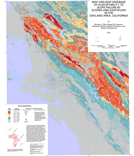
Map data that predict the varying likelihood of landsliding can help public agencies make informed decisions on land use and zoning. This map, prepared in a geographic information system from a statistical model, estimates the relative likelihood of local slopes to fail by two processes common to an area of diverse geology, terrain, and land use centered on metropolitan Oakland. The model combines the following spatial data: (1) 120 bedrock and surficial geologic-map units, (2) ground slope calculated from a 30-m digital elevation model, (3) an inventory of 6,714 old landslide deposits (not distinguished by age or type of movement and excluding debris flows), and (4) the locations of 1,192 post-1970 landslides that damaged the built environment. The resulting index of likelihood, or susceptibility, plotted as a 1:50,000-scale map, is computed as a continuous variable over a large area (872 km2) at a comparatively fine (30 m) resolution. This new model complements landslide inventories by estimating susceptibility between existing landslide deposits, and improves upon prior susceptibility maps by quantifying the degree of susceptibility within those deposits.
Susceptibility is defined for each geologic-map unit as the spatial frequency (areal percentage) of terrain occupied by old landslide deposits, adjusted locally by steepness of the topography. Susceptibility of terrain between the old landslide deposits is read directly from a slope histogram for each geologic-map unit, as the percentage (0.00 to 0.90) of 30-m cells in each one-degree slope interval that coincides with the deposits. Susceptibility within landslide deposits (0.00 to 1.33) is this same percentage raised by a multiplier (1.33) derived from the comparative frequency of recent failures within and outside the old deposits. Positive results from two evaluations of the model encourage its extension to the 10-county San Francisco Bay region and elsewhere. A similar map could be prepared for any area where the three basic constituents, a geologic map, a landslide inventory, and a slope map, are available in digital form. Added predictive power of the new susceptibility model may reside in attributes that remain to be explored—among them seismic shaking, distance to nearest road, and terrain elevation, aspect, relief, and curvature.
Susceptibility is defined for each geologic-map unit as the spatial frequency (areal percentage) of terrain occupied by old landslide deposits, adjusted locally by steepness of the topography. Susceptibility of terrain between the old landslide deposits is read directly from a slope histogram for each geologic-map unit, as the percentage (0.00 to 0.90) of 30-m cells in each one-degree slope interval that coincides with the deposits. Susceptibility within landslide deposits (0.00 to 1.33) is this same percentage raised by a multiplier (1.33) derived from the comparative frequency of recent failures within and outside the old deposits. Positive results from two evaluations of the model encourage its extension to the 10-county San Francisco Bay region and elsewhere. A similar map could be prepared for any area where the three basic constituents, a geologic map, a landslide inventory, and a slope map, are available in digital form. Added predictive power of the new susceptibility model may reside in attributes that remain to be explored—among them seismic shaking, distance to nearest road, and terrain elevation, aspect, relief, and curvature.
Pike, R.J., and Sobieszczyk, Steven, 2002, A Digital map of susceptibility to large landslides in Santa Clara County, California. Abstracts, EOS. Trans. AGU, v. 83, no. 47
Hillsides bordering the Santa Clara ("Silicon") Valley are prone to earthquake- and rainfall-triggered landslides. To narrow the uncertainty surrounding the location of future slope movement, we estimate the relative likelihood of landsliding at 30-m resolution from regional data sets. While small areas are evaluated accurately from detailed observations on material properties, topography, and hydrology, resource limitations force a regional, statistical, approach to mapping large areas. This is the first county-size susceptibility map prepared from the Arc/Info GIS model developed by Pike and others (2001) in the Oakland, CA, area (USGS MF-2385). Their index of susceptibility is the spatial frequency of prior slope failure for each one-degree slope interval in each geologic-map unit, obtained by combining a geologic map (a proxy for rock or soil strength) with a landslide-inventory map and a map of slope gradient. Areas in existing landslides are multiplied by an observationally derived constant, 1.33, to reflect their higher susceptibility. Santa Clara County's 170 geologic units occupy about 3,440,000 30-m grid cells. The geology is from three digital USGS maps (OF 97-710, 98-348, 98-795). The thousands of existing landslides were digitized from 13 inventories--six by the California Geological Survey, five by USGS, two by private consultants. These source maps vary in scale (mostly 1:24,000 or 1:12,000), date (1970-98), attribution of failures (most are large rock and debris slides, rock slumps, and earth flows; few are debris flows), completeness, and detail. The map of slope gradient (OF 98-766) was computed from a 30-m digital elevation model (OF 98-625). Severity of prior landsliding throughout the county strongly reflects geology--from a mean spatial frequency of zero, e.g. flat-lying Pleistocene alluvial fan and fluvial deposits, to 100%, e.g. a mudstone member of the Oligocene-Eocene San Lorenzo Formation. Values of the susceptibility index, ranging from zero (1,000,000 cells largely on the valley floor) to 1.33 (4200 cells in the most hazardous terrain), are not randomly distributed. Among large areas of highest susceptibility (>0.60) are the hills flanking Santa Clara Valley just E of the cities of San Jose, Milpitas, and Morgan Hill, as well as some terrain in the Santa Cruz Mountains.
Pike, R.J, Sobieszczyk, Steven, and Manning, C.D., 2003, A preliminary digital map of susceptibility to large landslides: International Landslide Research Group Newsletter, v. 17, digital note 1
BATHYMETRY & TERRAIN MODELS
Sobieszczyk, Steven, 2005, Digital Elevation Model of Scoggins Creek Drainage & Henry Hagg Lake
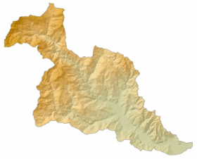
Available digital elevation models (DEMs) from USGS typically do not include the land surface topography (bathymetry) beneath the water surface of lakes and reservoirs. The Bureau of Reclamation (BOR) conducted a bathymetric survey of Henry Hagg Lake in 2001 and created a hypsography coverage from those bathymetric data. USGS personnel used Geographic Information Systems (GIS) to integrate the BOR bathymetric dataset with a USGS DEM of the topography above the lake's water surface. Using this newly combined surface dataset, a USGS water-quality model of Henry Hagg Lake was constructed to evaluate both current water quality and future scenarios in which the lake might be expanded.
Sobieszczyk, Steven, 2007, Digital Elevation Model of Detroit Lake
Available digital elevation models (DEMs) from the U.S. Geological Survey (USGS) typically do not include the land surface topography (bathymetry) beneath the water surface of lakes and reservoirs. USGS personnel used Geographic Information Systems (GIS) to create a DEM for Detroit Lake using topographic maps from the time period before Detroit Dam was built (1953). Those data were then merged with field data from a coarse lake bathymetric survey conducted by USGS personnel in 2002. Using this newly combined surface dataset, a USGS temperature and suspended sediment model of Detroit Lake was constructed to evaluate its circulation, thermal stratification, and transport and fate of suspended sediments.
URBAN INTENSITY
Falcone, James, Stewart, J.S., Sobieszczyk, Steven, Dupree J.A., McMahon, Gerard, and Buell, G.R, 2007, A comparison of natural and urban characteristics of the development of Urban Intensity Indices across six geographic settings: U.S. Geological Survey Scientific Investigations Report 2007-5123, 45p.
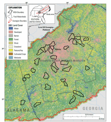
As part of the U.S. Geological Survey National Water- Quality Assessment Program, the effects of urbanization on stream ecosystems have been intensively investigated in six metropolitan areas in the United States. Approximately 30 watersheds in each area, ranging in size from 4 to 560 square kilometers (median is 50 square kilometers), and spanning a development gradient from very low to very high urbanization, were examined near Atlanta, Georgia; Raleigh, North Carolina; Denver, Colorado; Dallas-Fort Worth, Texas; Portland, Oregon; and Milwaukee-Green Bay, Wisconsin. These six studies are a continuation of three previous studies in Boston, Massachusetts; Birmingham, Alabama; and Salt Lake City, Utah. In each study, geographic information system data for approximately 300 variables were assembled to (a) characterize the environmental settings of the areas and (b) establish a consistent multimetric urban intensity index based on locally important land-cover, infrastructure, and socioeconomic variables. This paper describes the key features of urbanization and the urban intensity index for the study watersheds within each area, how they differ across study areas, and the relation between the environmental setting and the characteristics of urbanization. A number of features of urbanization were identified that correlated very strongly to population density in every study area. Of these, road density had the least variability across diverse geographic settings and most closely matched the multimetric nature of the urban intensity index. A common urban intensity index was derived that ranks watersheds across all six study areas. Differences in local natural settings and urban geography were challenging in (a) identifying consistent urban gradients in individual study areas and (b) creating a common urban intensity index that matched the site scores of the local urban intensity index in all areas. It is intended that the descriptions of the similarities and differences in urbanization and environmental settings across these study areas will provide a foundation for understanding and interpreting the effects of urbanization on stream ecosys- tems in the studies being conducted as part of the National Water-Quality Assessment Program.
LANDSLIDE INVENTORY
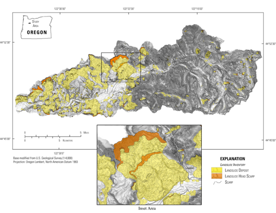
Sobieszczyk, Steven, 2010, Landslide inventory for the Little North Santiam River Basin, Oregon. U.S. Geological Survey, Dataset
Sobieszczyk, Steven, 2010, Top of head scarp and internal scarps for the landslide deposits in the Little North Santiam River Basin, Oregon. U.S. Geological Survey, Dataset
Sobieszczyk, Steven, 2010, Head scarp boundary for the landslides in the Little North Santiam River Basin, Oregon. U.S. Geological Survey, Dataset
Sobieszczyk, Steven, 2010, Location of photographs showing landslide features in the Little North Santiam River Basin, Oregon. U.S. Geological Survey, Dataset
ORGANIC BIOMASS

Sobieszczyk, Steven, 2011. Geomorphic floodplain with organic matter (biomass) estimates for Fanno Creek, Oregon. U.S. Geological Survey, Dataset
Sobieszczyk, Steven, 2011. Land cover classification for Fanno Creek, Oregon. U.S. Geological Survey, Dataset
Sobieszczyk, Steven, 2011. Normalized Difference Vegetation Index for Fanno Creek, Oregon. U.S. Geological Survey, Dataset
Sobieszczyk, Steven, 2011. Active channel for Fanno Creek, Oregon. U.S. Geological Survey, Dataset
Sobieszczyk, Steven, 2011. Water sample locations for Fanno Creek, Oregon. U.S. Geological Survey, Dataset
Sobieszczyk, Steven, 2011. SoiL sample locations for Fanno Creek, Oregon. U.S. Geological Survey, Dataset
Sobieszczyk, Steven, 2011. Stream Centerline for Fanno Creek, Oregon. U.S. Geological Survey, Dataset
POLLUTION IN THE PACIFIC NORTHWEST
SOBIESZCZYK, STEVEN, 2011, Location of Septic Sewer Systems in the Pacific Northwest, U.S. GEOLOGICAL SURVEY, DATASET
Sobieszczyk, Steven, 2011, Nutrient Impaired 303(d) Streams for the Pacific Northwest, U.S. Geological Survey, Dataset
Under section 303(d) of the 1972 Clean Water Act, states, territories, and authorized tribes are required to develop lists of impaired waters. These impaired waters do not meet water quality standards that states, territories, and authorized tribes have set for them, even after point sources of pollution have installed the minimum required levels of pollution control technology. The law requires that these jurisdictions establish priority rankings for waters on the lists and develop TMDLs for these waters” (U.S. Environmental Protection Agency, 2011). Waterways represented in this data set are a subset of these EPA 303 (d) listed streams that were classified as nutrient impaired. Nutrient impaired streams include those listed for nutrients, agriculture, crop sources, pH, dissolved oxygen, chlorophyll a, nitrate, phosphorus, and nitrogen. Total phosphorus and total nitrogen values attributed to stream reaches are based on EPA Level III Ecoregions aggregations for the National Nutrient Strategy values (U.S. Environmental Protection Agency, 2000). Values are based on 25th percentiles for aggregate nutrient reference conditions for both phosphorus and nitrogen. Data relate to a 2002 time period, with data collected from each of the state agencies as close to that period as possible.


